Indexing large vector embedding collections remains a pain point when setting up vector search infrastructures. Indexes like HNSW or IVF can take hours or even days to construct.
To tackle this issue, we have developed and open-sourced SuperKMeans, a super-fast clustering library for high-dimensional vector embeddings that drastically reduces indexing time from hours to mere seconds. In this blog post, I will show how SuperKMeans can index 10 million 1024-dimensional vector embeddings in just 1 minute on a single CPU. Additionally, I will explain the secret sauce behind SuperKMeans’s extremely fast clustering performance.
The dataset: I will be using the first 10M entries of the following dataset: https://huggingface.co/datasets/Cohere/msmarco-v2.1-embed-english-v3. This dataset contains MSMARCO passages embedded with the Cohere Embed V3 model, resulting in vector embeddings with a dimensionality of 1024. This is around 40 GB of information.
The index: We are going to build an IVF index with a point-per-cluster ratio of 1:256, resulting in approximately 40,000 centroids for our dataset.
The setup: For this experiment, I will be using a single Zen 5 machine equipped with 32 cores and 128 GB of RAM (m8a.8xlarge | $1.95/hr). However, it is worth noting that SuperKMeans works in any CPU (e.g., Intel’s, Graviton’s, Zen’s).
The code: You can find the script we used here. For this experiment, we used our C++ library. However, we also provide Python Bindings for ease of use and integration.
The results
The 10M vectors were indexed in just 68 seconds. These results are remarkable! Recall that we have achieved this on a single machine. Given that AWS charges for EC2 instances by the second, we have indexed 10 million vector embeddings for less than $0.04, at a remarkable rate of 150,000 vectors per second, or 0.61 GB per second!
For comparison, let’s run some benchmarks against a well-established vector clustering library: FAISS. In this experiment, we will compare SuperKMeans with a FAISS IVFFlat index. We will also use two versions of SuperKMeans: Vanilla SuperKMeans and Hierarchical SuperKMeans (we’ll explain the difference later!). The performance comparison is divided into two phases: i) computing the centroids, and ii) assigning all the points to their nearest centroid. These phases correspond to FAISS .train(), .add() API. The image below shows the results.
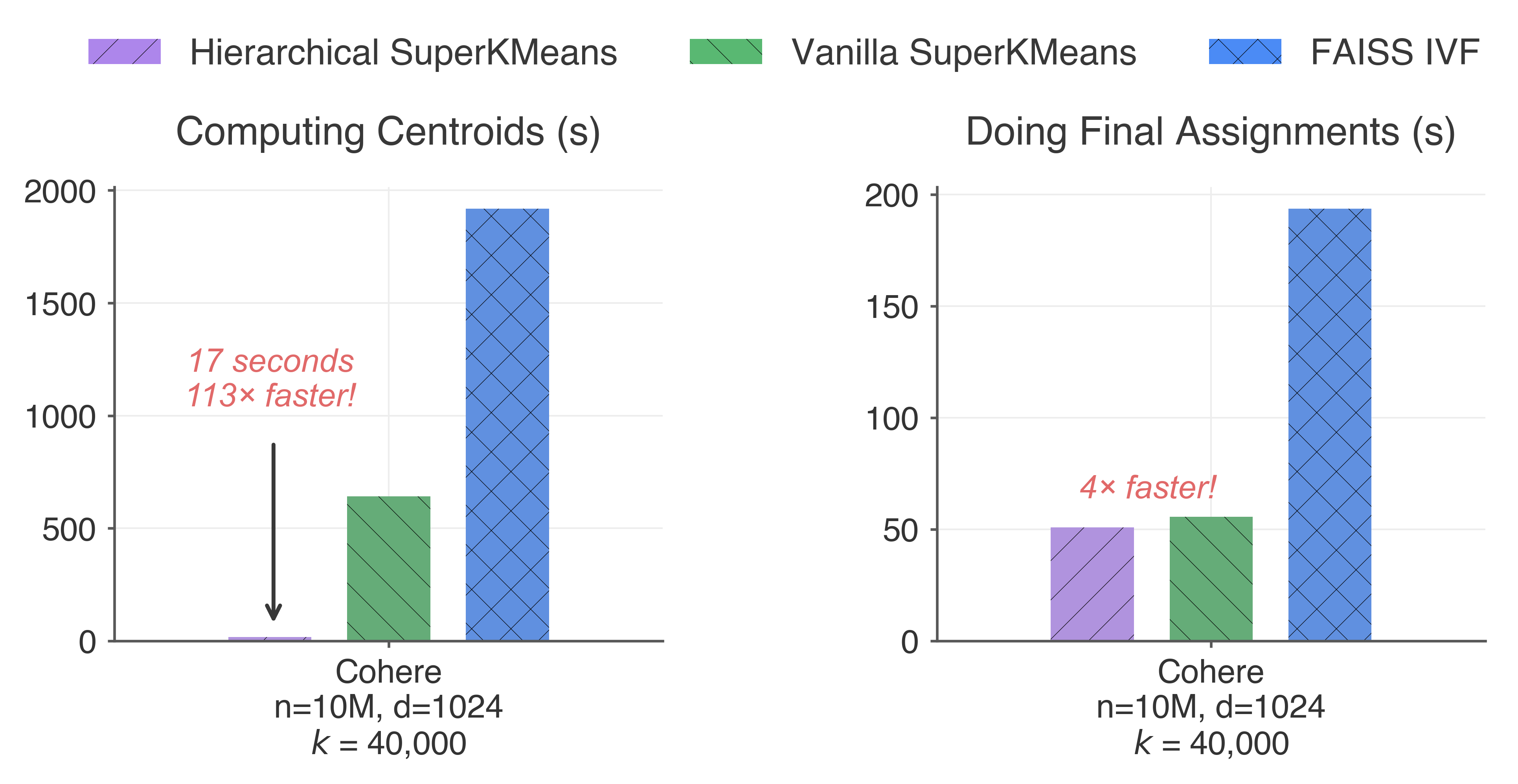
Hierarchical SuperKMeans is more than 100x faster than FAISS IVF to compute the centroids and 4x faster to perform the final assignments! Overall, Hierarchical SuperKMeans is 30x faster to index a vector collection from start to finish. Vanilla SuperKMeans also shows improved performance, with a 3x improvement over FAISS. Notably, in this experiment, both Vanilla SuperKMeans and FAISS do a fixed number of k-means iterations (10), and no data subsampling was performed.
But, is it a high-quality index?
Absolutely! Let’s compare the centroids obtained with SuperKMeans and FAISS in terms of their quality to fulfill vector search tasks. For this analysis, we used the recall@100 metric, measuring the recall obtained in the top-100 results while exploring 3% of the available clusters. We have also compared the balance of clusters by counting the number of distance calculations performed. The results are summarized in the table below:
| Algorithm | Indexing Time (s) | Recall@100 | Vectors Explored |
|---|---|---|---|
| FAISS IVF | 2113 | 0.956 | 33.5K |
| Vanilla SuperKMeans | 696 (3x faster) | 0.955 (equal) | 33.3K (equal) |
| Hierarchical SuperKMeans | 68 (30x faster) | 0.937 (-0.02) | 26.4K (21% less) |
The difference in recall@100 between FAISS IVF and Hierarchical SuperKMeans is minimal (around 2%). However, Hierarchical SuperKMeans significantly improves cluster balance while being 30x faster to construct. On the other hand, Vanilla SuperKMeans remains 3x faster to build!
The secret sauce
Now, let’s dive into the technical intricacies of the algorithm and explain why we are so fast. For the complete story, check out our scientific paper!
A, B, C of K-Means
First, let’s quickly recap what k-means is. K-means is a half-century-old algorithm for grouping multi-dimensional points into k clusters. In today’s context, it works exceptionally well for indexing vector embeddings. In a nutshell, k-means goes like this:
- Generate k initial centroids to initiate the algorithm.
- Assign each data point to its closest centroid.
- This requires computing a distance metric between each data point and centroid.
- Update the centroids based on the vectors assigned to them.
- Repeat steps 2 and 3 until the termination condition is met. This is the core loop of k-means.
- Finally, perform a last assignment of each point to its closest centroid.
Addressing the main bottleneck of k-means
The main bottleneck of the k-means algorithm is the calculation of distances between points and centroids. The most efficient way to do this is via matrix multiplication (GEMM), which is extremely optimized on modern hardware (e.g., in CPUs via BLAS libraries). In fact, GEMM is so optimized that k-means variants such as Elkan’s or Hammerly’s lose to Lloyd’s (vanilla) k-means, because they cannot interleave the matrix multiplication with the pruning of vectors. With SuperKMeans, we interleave a partial matrix multiplication with the pruning of distance calculations that are no longer needed to discard a centroid as an assignment to a vector. To do this efficiently, we implement the two-phase algorithm shown below:
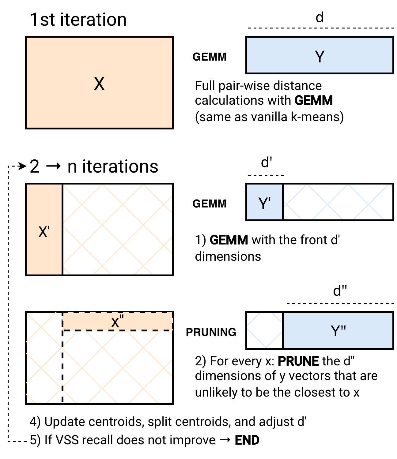
In the 1st iteration of k-means, we perform a full pairwise distance calculation. This is what every implementation of k-means does in every iteration. The following iterations are divided into two phases. The first phase (GEMM) performs pairwise distance calculations using optimized matrix-multiplication kernels on CPUs only for the front d' dimensions of the vector embeddings. Then, in the PRUNING phase, we avoid computing distances with centroids that are very unlikely to be a vector assignment. Notably, at the start of the PRUNING phase, more than 97% of the centroids are pruned, even with d' being as low as 12% of the dimensionality of the vectors. Thus, we efficiently avoid most of the computationally intensive work of k-means. This pruning effectiveness is thanks to a technique known as Adaptive Sampling (ADSampling), which, unlike other k-means variants (e.g., Elkan’s, Hammerly’s), performs progressive pruning rather than binary. Work is never wasted. Finally, to make the PRUNING phase even more performant, we adopt the recently proposed PDX layout for vector embeddings to achieve CPU-friendly pruning. This two-phased approach not only speeds up the core loop, but also the final assignment step.
There are more intricacies to the algorithm that you can check out in our paper. However, we will skip going too deep in the rabbit hole in this blog post.
Tuning hyperparameters for vector embeddings
Our findings reveal that to achieve high-quality centroids in vector embedding datasets:
- Running 5 to 10 iterations of the core loop is enough.
- Using 20-30% of the dataset is enough (though we benchmarked using the entire dataset).
- The more sophisticated initialization method, k-means++, is counterproductive rather than beneficial.
We have incorporated these insights into our library to optimize the quality-performance tradeoff when clustering vector embedding datasets.
Hierarchical K-Means: The cherry on top
We paired the idea of pruning with Hierarchical k-Means. In Hierarchical K-Means, we first run k-means to create √k meso clusters. Then, within each meso cluster, we run k-means again to create fine clusters that will serve as the centroids of our IVF index. Finally, we determine the final assignments by finding the closest centroid to each vector embedding. Throughout these phases, we use SuperKMeans to accelerate the pairwise distance calculation, the main bottleneck of the algorithm. The outcome? 10 million embeddings indexed in just 1 minute.
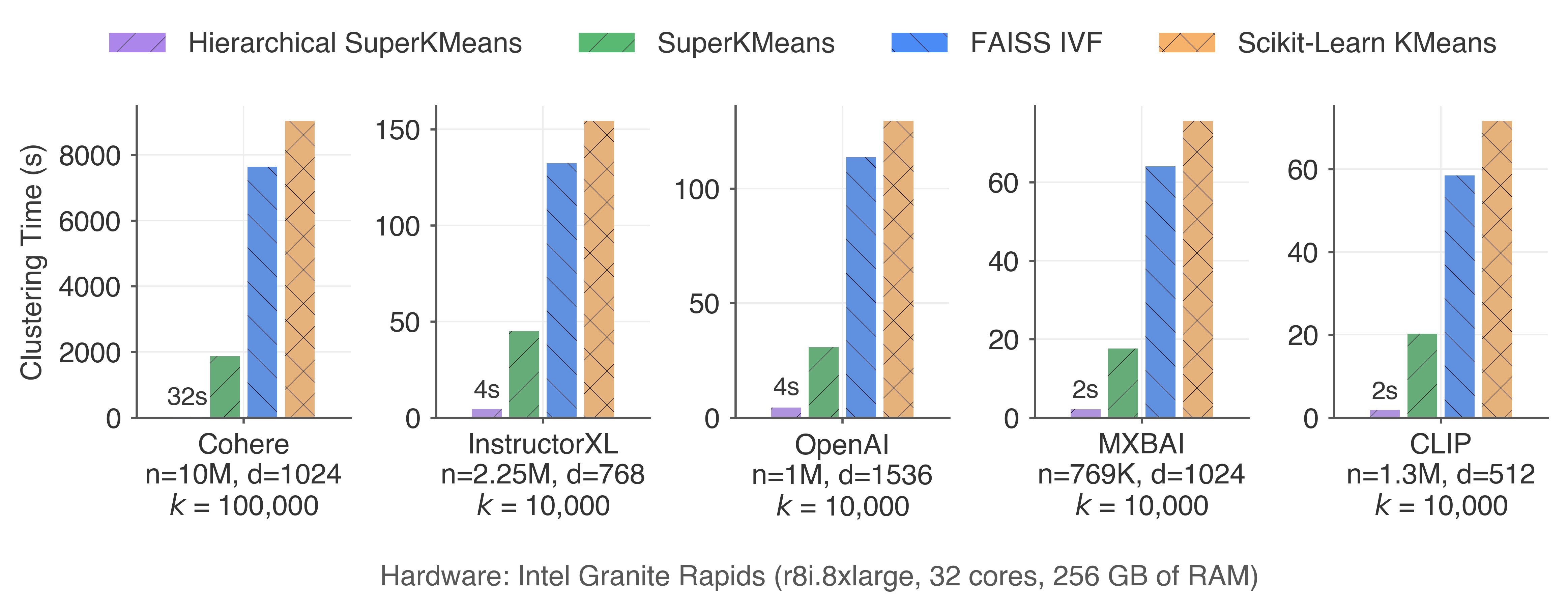
Other datasets
We have performed experiments with a variety of vector embedding datasets, using 5 CPU microarchitectures and GPUs. In every scenario, SuperKMeans outperforms conventional libraries for clustering embeddings. The advantages of SuperKMeans become even more pronounced with larger datasets or when using a lower points-per-cluster ratio.
Final remarks
SuperKMeans opens opportunities to reduce compute costs when creating partition-based indexes, such as IVF. We have shown that we can achieve extremely fast performance with a single machine, and without the need for GPUs.
Notably, we have also used the idea of dimension pruning in our standalone vector search library: PDX. In fact, I also have an extensive blog post about it. Pairing IVF indexes with PDX makes them competitive with heavyweight HNSW indexes. The figure below shows a queries-per-second (QPS) versus recall@10 curve comparing PDX+IVF, vanilla IVF with FAISS, and HNSW with USearch in the well-known OpenAI dataset of 1M embeddings of 1536 dimensions. For HNSW construction, we set ef_construction=128 and M=16. For IVF construction, we sample 30% of the data and set the number of clusters to 4000. Here, we are using Vanilla SuperKMeans to compare fairly against FAISS’ IVF.
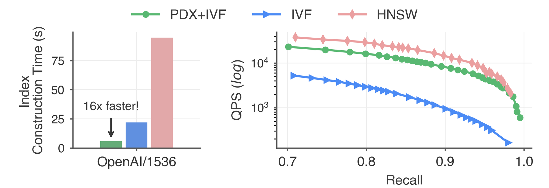
These results are groundbreaking, especially considering that IVF has traditionally been viewed as significantly slower than HNSW. In a nutshell, with PDX and SuperKMeans, we can now create an IVF index orders of magnitude faster than an HNSW index, using 6x less storage while achieving comparable query latency.
The scientific paper of SuperKMeans is available in arXiv.
Next stop: Billion-scale indexing in 1 minute ;)